see the blog at https://www.probabilitycourse.com/chapter6/6_2_5_jensen's_inequality.php

Remember that variance of every random variable $X$ is a positive value, i.e.,

Thus,

If we define $g(x)=x^2$, we can write the above inequality as \(E[g(X)] \geq g(E[X])\)

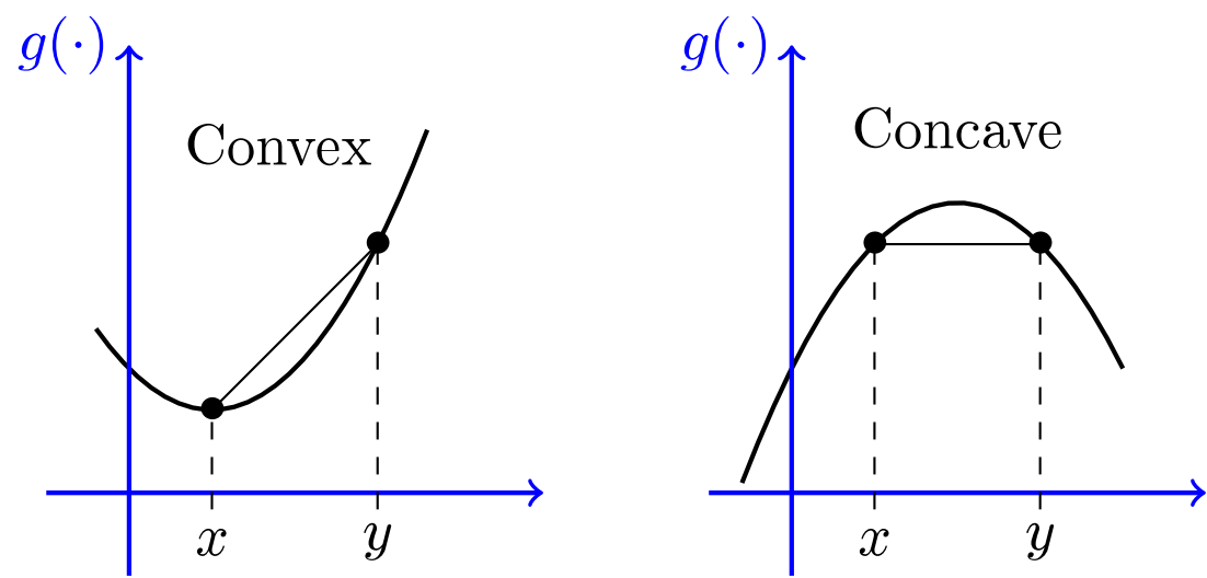
The function $g(x)=x^2$ is an example of convex function. Jensen’s inequality states that, for any convex function $g$, we have $E[g(X)] \geq g(E[X])$.

So what is a convex function? Figure below depicts a convex function. A function is convex if, when you pick any two points on the graph of the function and draw a line segment between the two points, the entire segment lies above the graph. On the other hand, if the line segment always lies below the graph, the function is said to be concave. In other words, $g(x)$ is convex if and only if $−g(x)$ is concave.

We can state the definition for convex and concave functions in the following way:

Convex and Concave Function Definition

Consider a function $g: \mathbf{I} \rightarrow \mathbb{R} $ , where $\mathbf{I} $ is an interval in $\mathbb{R}$. We say that $g$ is a convex function if, for any two points $x$ and $y$ in $\mathbf{I}$ and any $\alpha \in [0,1]$, we have \(g(\alpha x + (1−\alpha) y) \leq \alpha g(x) + (1− \alpha) g(y)\)

We say that $g$ is concave if \(g(\alpha x + (1−\alpha) y) \geq \alpha g(x) + (1− \alpha) g(y)\)

Note that in the above definition the term $\alpha x + (1−\alpha) y$ is the weighted average of $x$ and $y$. Also, $\alpha g(x) + (1− \alpha) g(y)$ is the weighted average of $g(x)$ and $g(y)$. More generally, for a convex function $ g: \mathbf{I} \rightarrow \mathbb{R}$ , and $x_1$, $x_2$, … , $x_n$ in $\mathbf{I}$ and nonnegative real numbers $\alpha_i$ such that $\sum_i^n \alpha_i=1$, we have

If $n=2$, the above statement is the definition of convex functions. You can extend it to higher values of $n$ by induction.

Now, consider a discrete random variable $X$ with $n$ possible values $x_1$, $x_2$, …, $x_n$. In Eq 1, we can choose $\alpha_i=P(X=x_i)=P_X(x_i)$. Then, the left-hand side of Eq 1 becomes $g(E[X])$ and the right-hand side becomes $E[g(X)]$ (by LOTUS). So we can prove the Jensen’s inequality in this case. Using limiting arguments, this result can be extended to other types of random variables.

Jensen’s Inequality Definition

If $g(x)$ is a convex function on $\mathbf{R}_X$, and $E[g(X)]$ and $g(E[X])$ are finite, then

Similarly, if $g(x)$ is a concave function, then we have

To use Jensen’s inequality, we need to determine if a function $g$ is convex. A useful method is the second derivative.

A twice-differentiable function $g: \mathbf{I} \rightarrow \mathbb{R}$ is convex if and only if $g″(x) \geq 0$ for all $x \in \mathbf{I}$.

For example, if $g(x)=x^2$, then $g″(x)=2 \geq 0 $, thus $g(x)=x^2$ is convex over $\mathbb{R}$.